

Sources of the Earth's magnetic field
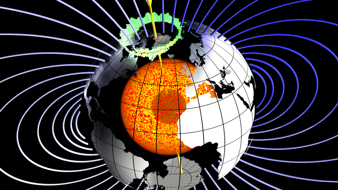
The dominant geomagnetic core field is generated in the Earth fluid outer core. The second part is generated by magnetized lithospheric rocks. A further contribution with a high temporal variety originates from sources outside of the Earth (Externel Field). Probably the faintest contribution to the Earth's magnetic field, is generated by oceanic circulations. More information about:
To fully describe the geomagnetic field it is necessary to either measure the intensity and two angles of direction or three orthogonal components. The angles are declination (the deviation of the local geomagnetic field lines from geographic north) and inclination (the angle of intersection with the Earth's surface). Orthogonal components are commonly chosen to be X, Y and Z for the directions towards geographic north, east and vertically down, respectively. Common units used to describe the geomagnetic field are nanoTesla (nT=10-9T) or microTesla (µT=10-6T) , with Tesla in fact being the unit for magnetic flux density.
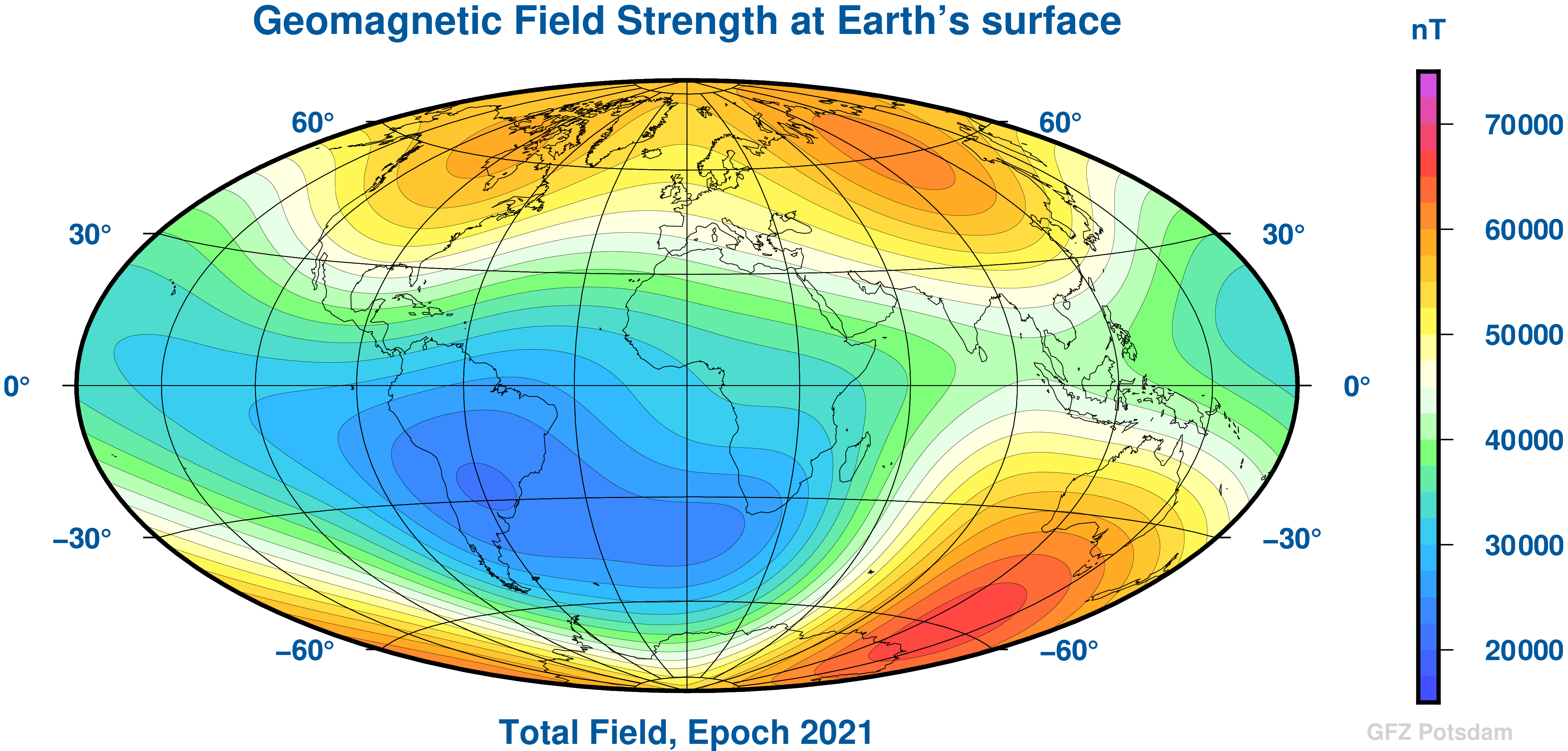
When a measurement of the geomagnetic field is taken at any given point and time, the resulting value contains the superposition of fields having different origins and varying in magnitude: the core field, the lithospheric field, the external fields and the electromagnetically induced field. In 1838 Gauss, using spherical harmonic functions, developed a method to describe the geomagnetic field globally, providing a rough separation between internal and external contributions to the geomagnetic field. Geomagnetic field models based on spherical harmonics are still widely used, but due to the multitude of sources, a strict separation of all contributions is not feasible. The following figure shows a map of the field strength distribution from such a model of the core field calculated from data from the CHAMP and Swarm satellites and from ground based geomagnetic observatories. An interesting feature of the core field is the so-called South Atlantic Anomaly. This is a large area of very low field intensity (less than 20µT) over South America, the southern Atlantic and southern Africa.
The core field is also subject to temporal variations, known as secular variation. From CHAMP(2006) and Swarm (2016) data we can see that the field has been decreasing further in parts of the South Atlantic Anomaly by up to 3.5 during the past 10 years. However, it is obvious that the magnetic field does not change uniformly over the Earth. While the overall strength of the dipole field is decreasing, there exist a few regions where the field strength is increasing, e.g. over the Indian Ocean and Europe.
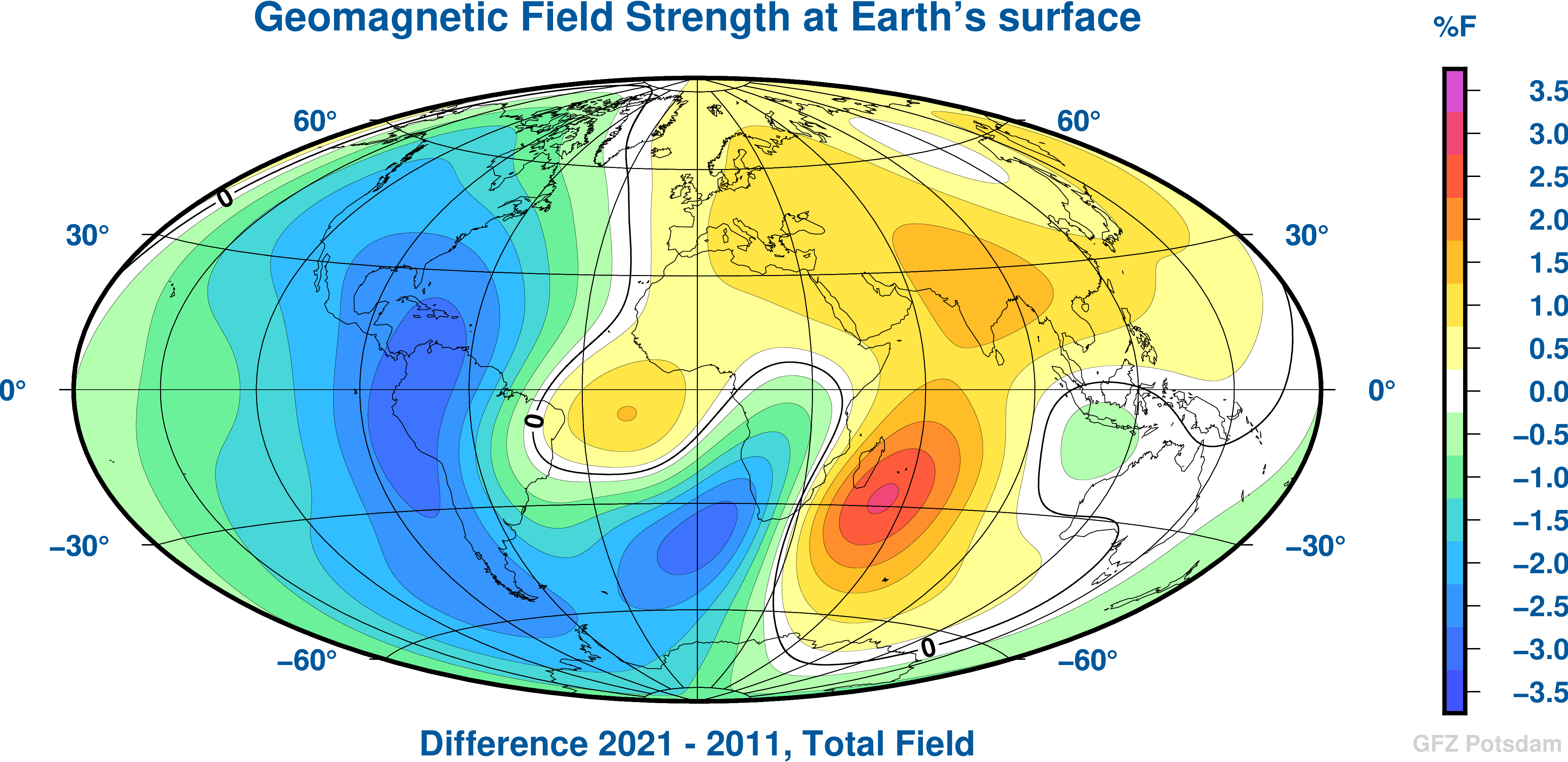
Modeling the secular variation on characteristic timescales of the order of a few decades, can be significantly improved if we take advantage of all the available magnetic satellite data. It is obvious that the magnetic field does not change uniformly over the Earth. While the overall strength of the dipole field is decreasing, there exist a few regions where the field strength is increasing. An extremely strong decrease is seen in two areas, in the South Atlantic and in the Meso-American region. From the 2011 and 2021 model data, we see that the field strength in the South Atlantic region has decreased by up to 3.5% over the last 10 years (see the following figure).
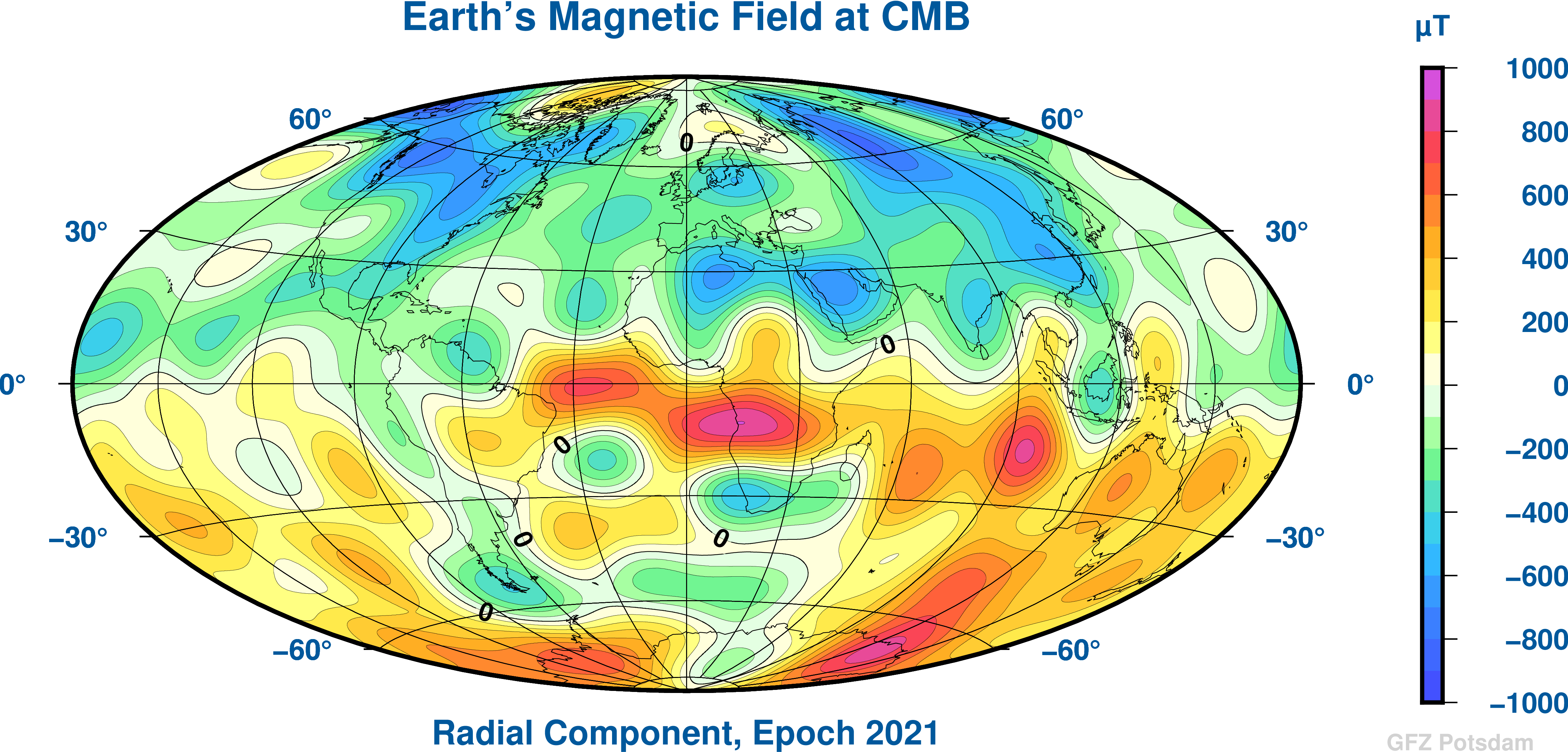
The field component used to probe the structure and dynamics of the Earth's core is the vertical component. Considering the mantle as an electrical insulator, the vertical component can be extrapolated to the core-mantle boundary, where its structure is more complicated than at the Earth's surface (see figure below). Distinct patches of reversed magnetic flux at the poles and below the South Atlantic region can be identified, which can be related to the present day field decrease. The most prominent feature in this respect is the growing patch of reverse magnetic polarity beneath the South Atlantic region.


The magnetization of the lithosphere is due to magnetic minerals, primarily magnetite with varying content in titanium. The titano-magnetite rich rocks become essentially non-magnetic above Curie temperatures of 400°C - 600°C and therefore, the lithospheric magnetization is limited to a layer of about 10km to 50km in thickness, depending on the local heat flow. The rock magnetization can be either induced (i.e. the magnetization is proportional to an inducing field, generally well approximated by the Earth's core field) or remanent when the magnetization strength and direction are "frozen in" the rocks and change only on very long time scale.
This lithosphere magnetization gives rise to a magnetic field which strength can be as large as several thousands of nT for the major anomalies like Kursk and Bangui, but in general is not much larger than 100nT. The lithospheric magnetic field is mapped by land, marine or airborne surveys and also from near-Earth satellite missions. A very large amount of marine and aeromagnetic surveys have been made at different epochs, over national or regional areas. However, the global mapping of the lithospheric magnetic field is possible only from satellite and has started with the POGO (1967-1971) and MAGSAT (1979-1980) missions. After 20 years without suitable measurements, significant progress have been made since 1999 with the high-quality data sets provided by the Oersted, SAC-C and CHAMP satellites.
For the lithospheric magnetic field, only wavelengths shorter than 2500km are visible. The longer wavelengths are overshadowed by the much stronger Earth's core field. What is generally referred to as the lithospheric magnetic field anomaly is actually only its short wavelength part. As the strength of a short wavelength anomaly decreases rapidly away from its source, the resolution of satellite data is limited to wavelengths longer than 400km; models of the lithospheric field for wavelength ranging from 400km to 2500km are now available. Information on shorter wavelength features are available only through marine or aeromagnetic surveys, or compilations of such surveys. A significant effort of the international geomagnetic community to merge together all available survey data lead to the first World Digital Anomaly Map, published in July 2007 (include WDMAM)

One contribution to the magnetic field of the Earth often varying rapidly in time and space has its sources in near Earth space. These magnetic signatures are from electric current systems in the magnetosphere and ionosphere, driven by solar radiation or thermospheric winds.

During quiet periods the amplitude of these external contributions are about 20 nT at mid-latitudes, increasing to more than ten- or hundred-fold during geomagnetic storms at all latidudes. The quantification of these geomagnetic sources allows the investigation of the near Earth space.
Projects
- SWAMI - Space Weather Atmosphere Model and Indices
- A global diagnosis of vertical atmospheric coupling by geomagnetic field variations
- Separating multidecadal internal geomagnetic secular variation and long-term magnetospheric field variations
- Main field influence on equatorial ionosphere
- Spatial and temporal structures of equatorial F region plasma depletions
- Swarm-AEBS - Auroral Electrojet and auroral Boundaries estimated from Swarm observations

The monitoring of ocean currents is of primary importance for understanding sea water quality, climate change and the global CO2 budget. Currently, global monitoring of ocean currents relies mainly on satellite radar measurements of the dynamic sea surface height. From two years of high precision CHAMP satellite magnetic measurements it has now been found possible to map the magnetic signal of ocean tidal flow. Movement of the highly conductive sea water through the Earth's magnetic field induces electric fields and currents, similar to a dynamo. The electric currents generate secondary magnetic fields which have been identified in the CHAMP satellite data. See:
Science, January 10, 2003, Volume 299, pp. 239-241.
Apart from opening new opportunities in the monitoring of ocean flow, the inclusion of ocean flow magnetic fields in our geomagnetic field modeling will raise the detectability of small scale crustal magnetisation.