

GFZ models of the Earth's Magnetic Field

Data based magnetic field models provide descriptions of the geomagnetic field and its evolution for each location on Earth and are used to study the underlying processes.
We develop and contribute to global and regional models of the Earth’s internal magnetic field. These include core field models for recent and long time scales based on observational or paleomagnetic data and lithospheric field models using satellite, aeromagnetic and ground data.

Mag.num models are the series of recent GFZ high-precision geomagnetic core field models that rely on satellite magnetic field measurements, in particular on calibrated Swarm and CHAMP vector field and ground observatory data. The coefficients of the spherical harmonic expansion is represented in snapshots and the temporal evolution between the snapshots is realised through spline interpolation. The coefficient files follows a dedicated formatfor Swarm magnetic field models.
Updates of Mag.num models are triggered by new satellite or observatory data, and will regularly be made available.
Coefficient tables of the Mag.num models:
- Mag.num-1:
- Mag.num-2:
- Mag.num.IGRF13 (GFZ IGRF-13 candidate parent model) 11/2013 - 09/2019, Swarm and ground observatories
- most recent, xx/xxxx - xx/xxxxx, Swarm and ground observatories (coming soon)
- Mag.num-3:
- current, Swarm satellite delta data only, xx/xxxx - xx/xxxx (along-track [Swarm A, B, C] and cross-track [Swarm A, C]) (coming soon)
CALS10k.2
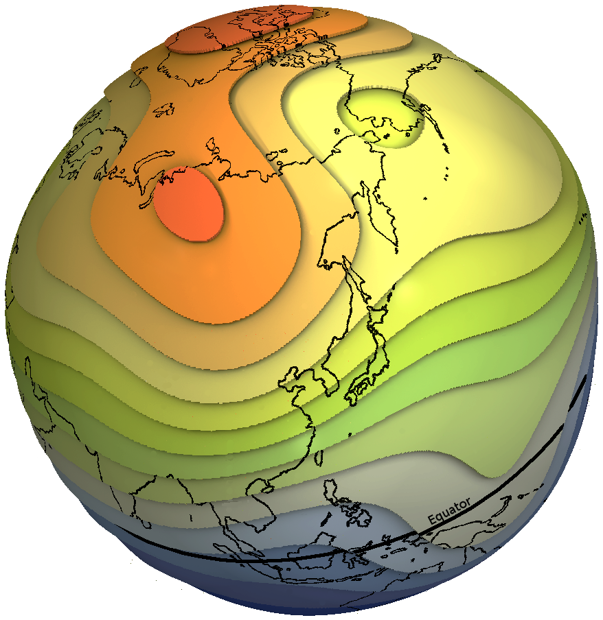
This updated version of geomagnetic field description for the past 10 000 years is mainly based on the same data as CALS10k.1b. However, the model offers higher temporal and spatial resolution due to improved uncertainty estimates for the data and calibrations of sediment relative paleointensity. The large-scale field at the core-mantle boundary and the Earth’s surface is described better by this model than by the previous version CALS10k.1b.
Reference:
- Constable, C., M. Korte and S. Panovska (2016): Persistent high paleosecular variation activity in Southern hemisphere for at least 10 000 years. Earth Planet. Sci. Lett.,453,78-86.
Downloads:
CALS10k_2.zip, 380 KB, Aug 2016, Model file CALS10k.2 with Fortran source code to obtain time series of field predictions at the Earth's surface (CALS10kfield.f) and to obtain the GAUSS coefficients for one point in time (CALS10kcoefs.f).
CALS10k_2_anim.zip, 48 MB, Aug 2016, Animations of radial field component (Br) at the core-mantle boundary and of field intensity at the Earth's surface.
DM_CALS10k_2.zip, 23 KB, Aug 2016, Plain text file with dipole moment estimate from CALS10k.2.
CALS10k.1b
We have used a comprehensive data compilation and recently refined modelling strategies to produce CALS10k.1b, the first time-varying spherical harmonic geomagnetic field model spanning 10 ky. The model is an average obtained from bootstrap sampling to take account of uncertainties in magnetic components and ages in the data (and hence has version number 1b instead of 1). This model shows less spatial and temporal resolution than earlier versions for 0 - 3 ka, and particularly aims to provide a robust representation of the large-scale field at the core-mantle boundary (CMB).
Reference:
- Korte, M., C. Constable, F. Donadini and R. Holme (2011): Reconstructing the Holocene Geomagnetic Field. Earth Planet Sci. Lett., 312, 497-505
Downloads:
CALS10k_1b.zip, 750 kB, Dec 2011, Model file CALS10k.1b with Fortran source code to obtain time series of field predictions at the Earth's surface with uncertainty estimates (CALS10kfield.f) and to obtain the GAUSS coefficients for one point in time (CALS10kcoefs.f).
CALS10k_1b_anim.zip, 33MB, Dec. 2011, Animations of radial field component (Br) at the core-mantle boundary and of field intensity at the Earth's surface.
DM_CALS10k_1b.zip, 80kB, Dec. 2011, Plain text file with dipole moment estimate from CALS10k.1b.
CALS3k.4 and CALS3k.4b
Global geomagnetic field reconstructions on millennial time scales can be based on comprehensive paleomagnetic data compilations but, especially for older data, these still suffer from limitations in data quality and age controls as well as poor temporal and spatial coverage. Here we present updated global models for the time interval 0 - 3 ka where additions to the data basis mainly impact the South-East Asian, Alaskan, and Siberian regions. Bootstrap experiments to generate uncertainty estimates for the model take account of uncertainties in both age and magnetic elements and additionally assess the impact of sampling in both time and space. Based on averaged results from bootstrap experiments, taking account of data and age uncertainties, we distinguish more conservative model estimates CALS3k.nb representing robust field structure at the core–mantle boundary from relatively high resolution models CALS3k.n for model versions n = 3 and 4. We presently consider CALS3k.4 the best high resolution model and recommend the more conservative lower resolution version for studies of field evolution at the CMB.
Reference:
- Korte, M. and C. Constable (2011): Improving geomagnetic field reconstructions for 0 - 3ka. Phys. Earth Planet. Int., 188, 247-259
Downloads:
cals3k-4.zip, 2.7MB, Nov. 2011, Four ASCII files with coefficients: CALS3k.4, CALS3k.4b, CALS3k.3, CALS3k.3b. Fortran source code fieldpred3k.f to produces time series of declination, inclination and intensity for any location on the Earth's surface from any of the four models, and fielduncert3k.f to produces time series with uncertainty estimates based on the bootstrap from models CALS3k.4b or CALS3k.3b.
CALS3k-4anim.zip, 3.9MB, Nov. 2011, Animations of radial field component (Br) at the core-mantle-boundary as predicted by the four models and of the radial field differences between model versions 3 and 4.
CALS3k, ARCH3k, SED3k
This series of 5 main field models spanning the past 3kyrs was created to obtain a better understanding of the possibilities and limitations offered by different data types to reconstruct the global geomagnetic main field of the Holocene. Archeomagnetic data are generally considered to offer smaller uncertainties and particularly better age control than sediment records. Moreover, sediment records can at most provide information on relative intensity variation, but not on absolute paleointensity. On the other hand, archeomagnetic data are sparse prior to 1000 BC and from the southern hemisphere in general. Longer term global field reconstructions necessarily have to rely on sedimentary data, and even 3kyr models based only on archeomagnetic data are biased by the hemispherically assymmetric data distribution. Details are given in the references below. We conclude that models based on all available data, both archeomagnetic and sediments like in CALS3k.3, at present provide the most reliable reconstruction of the past geomagentic field evolution.
The five models are:
- CALS3k.3 based on all available data and with uncertainty estimates based on a bootstrap method.
- CALS3k_cst.1 based on all data types but with prior quality selection.
- ARCH3k.1 based only on archeomagnetic data and with uncertainty estimates based on a bootstrap method.
- ARCH3k_cst.1 based on archeomagnetic data with prior quality selection.
- SED3k.1 based only on sediment records where relative intensity has been scaled by the archeomagnetic model and with uncertainty estimates based on a bootstrap method.
References:
- Korte, M., F. Donadini and C. Constable (2009): Geomagnetic Field for 0-3ka: 2. A new Series of Time-varying Models. Geochem. Geophys. Geosys., 10, Q06008, doi:10.1029/2008GC002297
- Donadini, F., M. Korte and C. Constable (2009): Geomagnetic Field for 0-3ka: 1. New Data Sets for Global Modeling. Geochem. Geophys. Geosys., 10, Q06007, doi:10.1029/2008GC002295
Downloads:
CALS3k_3.zip, 1.5MB, May 2010, CALS3k_3 Model coefficients with uncertainty estimates and Fortran code for evaluation.
ARCH3k_1.zip, 30kB, May 2010, ARCH3k_1 Model coefficients with uncertainty estimates and Fortran code for evaluation.
SED3k_1.zip, 6.4MB, May 2010, SED3k_1 Model coefficients with uncertainty estimates and Fortran code for evaluation.
CALS3k_cst_1.zip, 6.5MB, May 2010, CALS3k_cst_1 Model coefficients and Fortran code for evaluation.
ARCH3k_cst_1.zip, 1.4MB, May 2010, ARCH3k_cst_1 Model coefficients and Fortran code for evaluation.
Dipole.zip, 700kB, May 2010, Dipole Text files with dipole moments (with uncertainties) for all 5 models.
The GGFSS70 is a global geomagnetic field model covering the period 70,000 to 15,000 years ago. The model is based on nine selected sediment records from globally distributed sites. The dataset contains only high-quality paleomagnetic records, with high temporal resolution (sedimentation rate) and good independent age control. It covers three geomagnetic excursions: Norwegian-Greenland Sea (65,000 years ago), Laschamps (41,000), and Mono Lake/Auckland (34,000). The model exhibits a better temporal resolution than the GGF100k model that covers the past 100,000 years.
Citation
- Panovska, S., Korte, M., Liu, J., & Nowaczyk, N. R. (2021). Global evolution and dynamics of the geomagnetic field in the 15-70 kyr period based on selected paleomagnetic sediment records. J. Geophys. Res. Solid Earth, 126, e2021JB022681. doi: 10.1029/2021JB022681
Downloads
- https://earthref.org/ERDA/2472/ model coefficients and codes
- https://earthref.org/ERDA/2471/ model animation
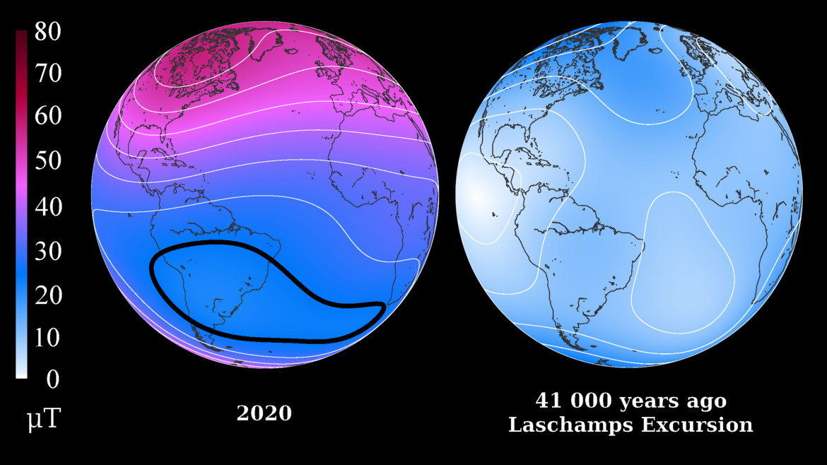
GGF100k is a global geomagnetic field model covering the past 100,000 years. It is the first model that provides a global view of the geomagnetic field evolution over an extended period. The model is based on an extensive global dataset of over 100 sediment records, and volcanic data. The geomagnetic axial dipole moment exhibits a broad range of variations, with the lowest value during the Laschamps excursion (41,000 year ago). Other excursions appear in limited locations and are likely regional events.
Citation
Panovska, S., Constable, C. G., & Korte, M. (2018). Extending global continuous geomagnetic field reconstructions on timescales beyond human civilization. Geochem. Geophys. Geosyst., 19. doi: 10.1029/2018GC007966
Panovska, S., Korte, M., & Constable, C. G. (2019). One hundred thousand years of geomagnetic field evolution. Rev. Geophys., 57. doi: 10.1029/2019RG000656
Downloads
- https://earthref.org/ERDA/2382/ model coefficients and codes
- https://earthref.org/ERDA/2384/ model animations
A Link to the Eos Editors’ Vox article by AGU: https://eos.org/editors-vox/the-global-geomagnetic-field-of-the-past-hundred-thousand-years
LSMOD Models
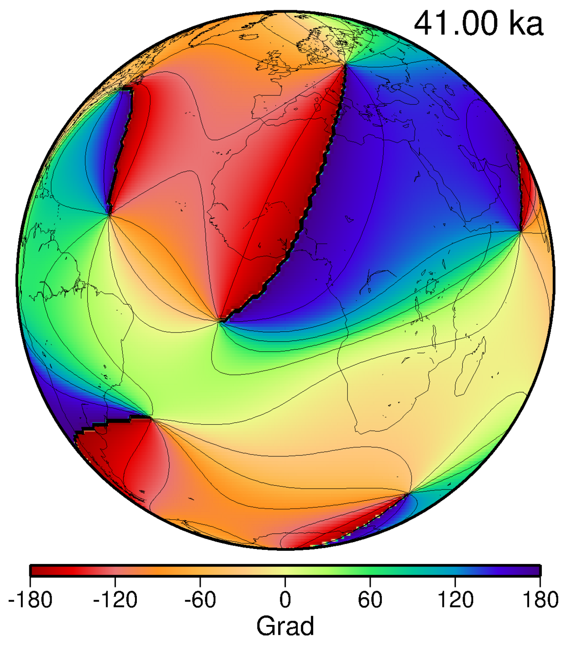
The LSMOD models (current version LSMOD.2) represent the global evolution of the geomagnetic field for the time interval 50 to 30 ka. They are based on paleomagnetic data from sediments and volcanic rocks. They contain the Laschamp excursion (ca. 41 ka), which is characterized by globally reversed field directions and very low field intensities, and the less pronounced Mono Lake excursion (ca. 33 ka).
Data from the first year of ESA's Swarm constellation mission are used to derive the Swarm Initial Field Model (SIFM), a new model of the Earth's magnetic field and its time variation.
GRIMM-3
The GFZ Reference Internal Magnetic Model release 3 (GRIMM-3) is mainly an improvement of GRIMM-2.
Downloads:
GRIMM-3_0.zip, 274 kB, Aug 2011, Fortran95 code for forward modelling for GRIMM-3.0 (development branch) and a single epoch model from GRIMM-3.0, coefficent file.
GRIMM-3_0.mov, 6,4 MB, March 2011, Movie of secular acceleration of the vertical down component of the Earth's core magnetic field.
GRIMM-2 (x)

The GFZ Reference Internal Magnetic Model (GRIMM2) has been derived from nearly eight years of CHAMP satellite data and seven years of observatory hourly means. At high latitudes, full vector satellite data are used at all local times. By doing so, a separation is possible between, on one hand, the fields generated by the ionosphere and field aligned currents, and, on the other hand, the fields generated in the Earth's core and lithosphere. This selection technique leads to a data set where gaps are avoided during the polar summers allowing the modelling of the core field with an unprecedented time resolution. Order six Bsplines are used to model the core field and the mapping of its acceleration is possible from 2001.5 to 2008.5 revealing a rapid and complex evolution over this time period at the Earth's surface. The energy in secular acceleration presents a smooth behaviour in time and is shown to increase continuously from 2003.5 to reach a maximum around 2006.0.. The static core field and its secular variation are all in good agreement with previously published magnetic field models.
Downloads
GRIMM-2.zip, 81 kB, July 2009, Fortran95 code for forward modelling for GRIMM-2 and a single epoch model from GRIMM-2, coefficent file.
GRIMM2x.zip, 89 kB, Oct. 2009, Fortran95 code for forward modelling for GRIMM-2x and a single epoch model from GRIMM-2x, coefficent file.
GRIMM-1

The GFZ Reference Internal Magnetic Model (GRIMM) has been derived from nearly six years of CHAMP satellite data and five years of observatory hourly means. At high latitudes, full vector satellite data are used at all local times. By doing so, a separation is possible between, on one hand, the fields generated by the ionosphere and field aligned currents, and, on the other hand, the fields generated in the Earth's core and lithosphere. This selection technique leads to a data set where gaps are avoided during the polar summers allowing the modelling of the core field with an unprecedented time resolution. Order five B-splines are used to model the core field and the mapping of its acceleration is possible from 2001.5 to 2005.5 revealing a rapid and complex evolution over this time period at the Earth's surface. The energy in secular acceleration presents a smooth behaviour in time and is shown to increase continuously from 2003.5. Due to the regularisation technique introduced, the acceleration energy for spherical harmonics 6 to 11 is significantly larger than for other available geomagnetic models. The static core field, its secular variation and the lithospheric field are all in good agreement with previously published magnetic field models.
Downloads
GRIMM_splines.zip ,36 kB, Jun 2007, GRIMM Gauss Coefficients SH degrees 1 to 14.
GRIMM_2003.5.zip, 147kB, Aug 2007, GRIMM Gauss Coefficients for the static core field, its secular variation and acceleration in 2003.5.
GJI-07-0346-R.pdf 5,1 MB, Feb 2008, GRIMM - The GFZ Reference Internal Magnetic Model based on vector satellite and observatory data (GJI, 2008).
The Digital Magnetic Anomaly Map of the World - WDMAM
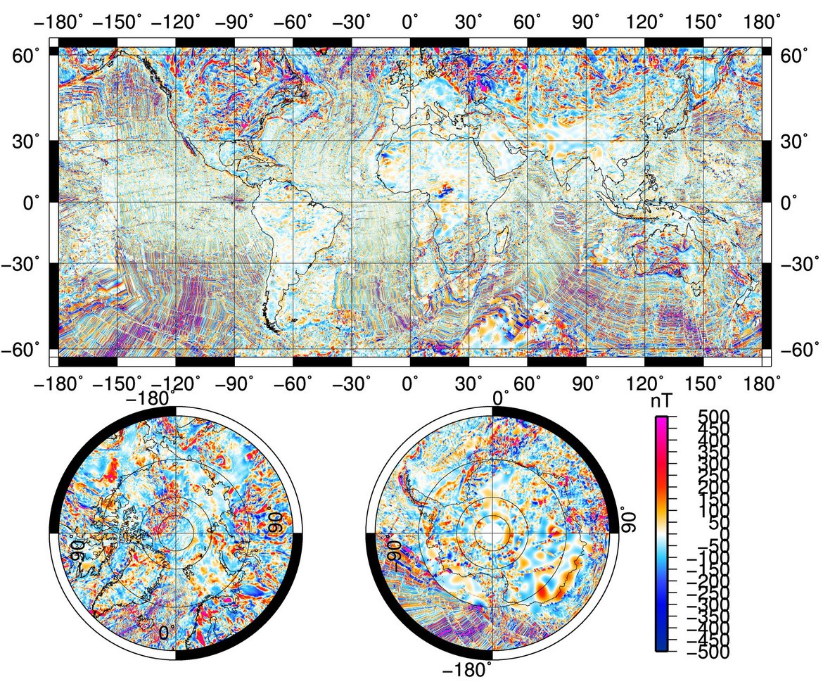
The Digital Magnetic Anomaly Map of the World (WDMAM) results from an international effort to build the first global compilation of the wealth of magnetic anomaly information derived from more than 50 years of aeromagnetic surveys over land areas, research vessel magnetometer traverses at sea, and observations from earth-orbiting satellites, supplemented by anomaly values derived from oceanic crustal ages. The objective is to provide an interpretive dimension to surface observations of the Earth's composition and geologic structure. The magnetic anomalies represented on this map originate primarily in igneous and metamorphic rocks, in the Eart's crust and possibly, uppermost mantle. Magnetic anomalies represent an estimate of the short-wavelength (<2600 km) fields associated with these parts of the Earth, after estimates of fields from other sources have been subtracted from the measured field magnitude. The natural increase of temperature with depth in the Earth means that rocks below a certain depth, termed the Curie depth, will be essentially non-magnetic. This depth is typically in excess of 20 km in stable continental regions, and may be as shallow as 2 km in young oceanic regions. Studies of crustal magnetism have contributed to geodynamic models of the lithosphere, geologic mapping, and natural resource exploration. Inferences from crustal magnetic field maps such as these, interpreted in conjunction with other information, can help delineate geologic provinces, locate impact structures, dikes, faults, and other geologic entities which have a magnetic contrast with their surroundings. To this end, the World Digital Magnetic Anomaly Map (WDMAM) is available in both digital and map form at CGMW and GTK.
The GFZ has been involved in the compilation of this map and has built its own version of the map that can be downloaded from GTK. As for the official map, the anomaly field is shown at an altitude of 5 km above the WGS84 ellipsoid. The magnetic fields shown are designed to be internally consistent over the measurement domain, extending from the surface to satellite altitude.
Downloads:
GMJC-Candidate-2.zip, 311MB, Sep 2014, Weltweite ASCII Raster-Datei (GRID) des WDMAM mit einer Auflösung von 0.05 Grad.
model_WDMAM.zip, 6,6MB, Sep 2014, WDMAM Modell Daten (gepackte ASCII-Datei).
WDMAM.jpg, 6,1MB, Sep 2014, Hochaufgelöste Bilddatei der WDMAM (4224x3500 Pixel).
INDEX.jpg, 6,1MB, Sep 2014
GRIMM_L, Version 0.0
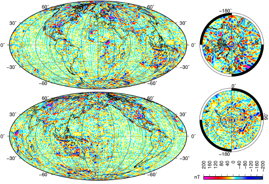
We investigated how the noise in satellite magnetic data affects magnetic lithospheric field models derived from these data in the special case where this noise is correlated along satellite orbit tracks. For this we describe the satellite data noise as a perturbation magnetic field scaled independently for each orbit, where the scaling factor has a specified variance. Under this assumption, we have been able to derive a model for errors in lithospheric models generated by the correlated satellite data noise. Unless the perturbation field is known, estimating the noise in the lithospheric field model is a non-linear inverse problem. We therefore proposed an iterative post-processing technique to estimate both the lithospheric field model and its associated noise model. The technique has been successfully applied to derive a lithospheric field model from CHAMP satellite data up to spherical harmonic 120. The model is in agreement with other existing models. The technique can be in principal extended for all kind of potential field data with ”along track” correlated errors.
The reference associated with the model is for now: http://www.solid-earth-discuss.net/4/1345/2012/sed-4-1345-2012.pdf
Downloads:
GRIMM_L120.coeff.zip, 110kB, Nov. 2012, List of Gauss coefficients for the lithospheric field model.
GRIMM_N120.coeff.zip, 193kB, Nov. 2012, Noise model subtracted.
FF-Model


The FF-model is a geomagnetic field model for epoch 2005.4 that has been built from one year of CHAMP and observatory data. In this model, the flow at the top of the liquid outer core is co-estimated together with the field model using the radial diffusion-less induction equation. The constraints are applied exclusively on the flow model. This approach leads to a magnetic field model that is compatible in time with the frozen-flux approximation. In particular, the field model acceleration at spherical harmonic degrees higher than 5 correspond to the acceleration that would be obtained for a static flow. This component of the acceleration is much weaker than the contribution due to the time variation of the flow (see Figure 1). It can be downward continued to the CMB (Figure 2).
Download:
FF-Model.zip, 3.9kB, July 2008, Gauss coefficients for year 2004.5.
Continuous Covariant Constrained-end-points field model - C3FM

This study presents an investigation and description of the secular variation of the Earth's magnetic field between 1980 and 2000. A time-dependent model, C³FM (Continuous Covariant Constrained-end-points Field Model), of the main field and its secular variation between 1980 and 2000 is developed, with Gauss coefficients expanded in time on a basis of cubic B-splines. This model is constrained to fit field models from high quality vector measurements of MAGSAT in 1980 and Ørsted in 2000 and to fit both magnetic observatory and repeat station secular variation estimates for the period in between. These secular variation estimates (first time derivatives) are derived from observatories monthly or annual means and repeat station data in order to reduce the contributions of crustal noise, annual and semi-annual variation. On average, the model input consists secular variation estimates of the X, Y and Z components at 130 locations per month. Treatment of covariance between the different components allows a higher temporal sensitivity of the model, due to the exclusion of some external field variation. The model is computed up to degree and order 15.
The model is a useful extension of the hitherto existing time-dependent description of the secular variation, GUFM which describes the secular variation until 1990. It reveals a short term secular variation on sub-decadal time scale and has a higher spatial resolution, than previously resolved. The model is also valuable to test the frozen flux hypothesis and to link features of the radial field at the core-mantle boundary to the geodynamo.
Downloads:
c3fm_spline.zip, 68kB, Aug. 2007, C3FM Gauss Coefficients SH degrees 1 to 15 (ASCII file containing spline).
c3fm_main_field.zip, 630kB, Aug. 2007, C3FM core field coefficients SH degrees 1 to 15 for each month during 1980 to 2000 (241 ASCII files).
c3fm_sec_variation.zip, 630kB, Aug. 2007, C3FM secular variation coefficients SH degrees 1 to 15 for each month during 1980 to 2000 (241 ASCII files).
c3fm_model_paper_preprint.pdf, 207kB, Aug. 2007, C3FM model paper preprint.
CHAOS-4, is a new version in the CHAOS model series, which aims to describe the Earth's magnetic field with high spatial and temporal resolution.
More than 14 years of data from the satellites Oersted, CHAMP and SAC-C, augmented with magnetic observatory monthly mean values have been used for this model.
